Convex Hypertree Based Reparametrization and Convex Upperbounds

To motivate why reparametrizations of probability distributions are important we first consider a simple scenario of exponenential family $p_{\theta}, \theta \in \Theta \in \R^{p}$ on a tree structured graph $G^T = (V^T,E^T)$. We already know one simple clique factorization (edge and nodes on $V^T$)

As we already know from the concepts of graphical models a major chalange of inference tasks is the access to partition function $Z$. Assumming for a moment that we have access to the marginals $p(x_v,x_w)$, then we can factorize $(1)$ directly in terms of the margnials via

where now due to the proper normalization of the marginals the partition function vanishes, i.e. $Z = 1$. Now given as exponential family with initial regular parametrization $\theta^{\\ast}$ leveraging factorization (2) implies

where the correspodning log partition function becomes $A(\theta^{\ast}) = 0$. In this way we can observe that instead computing normalization contansts we alternatively can seek for a reparametrization parameter $\theta^{\ast}$ which factorizes according to $(2)$. If the graph is a tree, such reparametrization is easely obtained by marginal inference via message passing updates in linear time. However, the major challenge is to define proper reparametrizations updates on graphs with cycles. This is due to the following reasons

• $(i)$ The geometry of the underlying parameter space $\Theta$ directly depends on the complex shape of the underlying marginal polytop, i.e. in the presence of cycles this is a highly contrained set.
• $(ii)$ Each reparametrization must index the same joint probability distribution, i.e. wee need access the global properties of the underlying distribution.

In turns out, that for a particular class of exponential families, the gloabl shape of distribution in $(ii)$ is reconstructed from a family of much simpler structures (chains, trees, hypertrees, etc.) which also yields approximations and error bounds to the marginal polytope in $(i)$

Inference Problems on Tree-Graphs and Bethe Approximation

We first consider a generall parametrization of exponential family (3)

$p\theta(x)\propto\exp\big\{\sum_{s\in V}\theta_{s}(x_{s})+\sum_{(s,t)\in E}\theta_{s t}(x_{s},x_{t})\big\},$

which arises from (3) for the particular choice of sufficient statistics given by overcomplete representation

$\theta_{s}(x_{s}):=\sum_{i}\theta_{s;j}\mathbb{1}_{s;j}(x_{s}), \qquad \theta_{s t}(x_{s},x_{t}):=\sum_{(j,k)}\theta_{s t;j k}\mathbb{1}_{s t;j k}(x_{s},x_{t})$

which is also commonly denoted as nonidentifable due to the existance of affine subpace $A^{\theta}$ such that $\theta \in A^{\theta}$ indexis the same distribution.

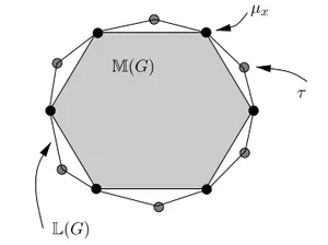
and introduce the set of all realizable marginals

$\mathbb{M}(G):=\{\mu\in\mathbb{R}^{d}\mid\exists\;p\;{\mathrm{with~marginals}}\;\mu_{s}(x_{s}),\,\mu_{s t}(x_{s},x_{t})\} \qquad (\text{Marginal Polytope}).$

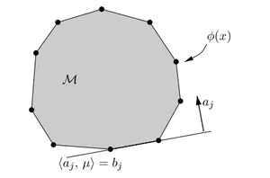
The above set is denoted as the marginal polytop and can equivalently be written as a convex hull over vector corresponding to each configuration $x$ or equivalently as an intersection over an exponential number of half spaces for each configuration.
If the graph is a tree (no cycles) it can be shown that the marginal polytope admits a much simpler characterization in terms of locally consistent marginal distributions $0 \leq \xi \in \mathbb{L}(G)$ which satisfy the pairwise marginalization constraints

$\sum_{x_{s}}\xi_{s}(x_{s})=1, \qquad \sum_{x_{t}^{\prime}}\xi_{s t}(x_{s},x_{t}^{\prime}) = \xi_{s}(x_{s}),\quad\forall\,x_{s}\in\mathcal{X}_{s}$

$\sum_{x_{t}^{\prime}}\xi_{s t}(x_{s},x_{t}^{\prime})\,=\,\xi_{s}(x_{s}),\quad\forall\,x_{s}\in\mathcal{X}_{s}, \qquad \sum_{x_{s}^{\prime}}\xi_{s t}(x_{s}^{\prime},x_{t})\,=\,\xi_{t}(x_{t}),\quad\forall\,x_{t}\in X_{t}$

An important observation is that if the graph is a tree than the two sets agree $\mathbb{M}(G) = \mathbb{L}(G)$ and in the presence of cycles $\mathbb{M}(G) \subset \mathbb{L}(G)$, i.e. it always serves as an upperbound to the complex marginal polytope.

In order to see the difference between the two sets let us consider a classical example of a one cycle graph $G = (\{1,2,3\},\{(12),(23),(31)\})$. For each parameter $\xi_{st}$ we consider variational marginals

$\xi_{s}(x_{s}):=\ [0.5\ \ \ 0.5] \qquad \xi_{s t}(x_{s},x_{t}):=\left[\begin{array}{c c}{{\tau_{s t}}}&{{0.5-\xi_{s t}}}\\ {{0.5+\beta_{s t}}}&{{\tau_{s t}}}\end{array}\right],$

which satisfy marginalization conditions and therefore $\xi \in \mathbb{L}(G)$. In order to seek for the corresponding joint distrubution $p(x_1,x_2,x_3)$ on graph $G$ with such marginals we check all the marginalization constraints while keeping the node marginals $\xi_1 = \xi_2= \xi_3 = \frac{1}{2}$ fixed.

$\xi_{s}(x_{s})\,=\,\sum_{x_{t}^{\prime},x_{u}^{\prime}}\xi_{s t u}(x_{s},x_{t}^{\prime},x_{u}^{\prime})\qquad \xi_{s t}(x_{s},x_{t})\,=\,\sum_{x_{u}^{\prime}}\xi_{s t u}(x_{s},x_{t},x_{u}^{\prime})$

which after small algebraic calculation can be reduced to the following set of inequalities

$\begin{array}{l}{{\displaystyle \xi_{s t u}\ge0}}\\ {{\displaystyle \xi_{s t u}\ge-\xi_{s}+\xi_{s t}+\xi_{t}+\xi_{s u}}}\\ {{\displaystyle \xi_{s t u}\le1-\xi_{s}+\tau_{t}+\xi_{s t}+\xi_{s t}+\xi_{s u}+\xi_{t u}}}\\ {{\displaystyle\xi_{s t u}\le\xi_{s t},\xi_{s u},\xi_{t u}.}}\end{array}$

Returning to our example the above set of inequalities boilds down to

$\begin{array}{l l}{{\xi_{12}+\xi_{23}-\xi_{13}\leq\frac{1}{2},}}&{{\xi_{12}-\xi_{23}+\xi_{13}\leq\frac{1}{2},}}\\ {{-\xi_{12}+\xi_{23}+\xi_{13}\leq\frac{1}{2},}}&{{\mathrm{and~}\quad \xi_{12}+\xi_{23}+\xi_{13}\leq\frac{1}{2}.}}\end{array}$

which illustrates how the marginal polytope is contained within the 3D cube $[0,\frac{1}{2}]^3$. Now after plugging in the expression for the local polytope it is easely seen that

$\tau_{12}+\tau_{23}-\tau_{13}\,=\,0.4+0.4-0.1\,\gt \,{\frac{1}{2}}.$

which shows that for $\tau_{st} = 0.4$ there exists no probability distribution on $\mathcal{G}$ with the marginal given by (add number ).

Bethe Entropy Approximation

Not only the marginal polytope on tree-structured graphs posesses a particular simple structure but also the Bethe entropy admits a closed form expression

$H(p_{\mu}) = \sum_{s\in V}H_{s}(\mu_{s})-\sum_{(s,t)\in E^T}I_{s t}(\mu_{s t}).$

with

$H_{s}(\xi_{s}):=-\sum_{x_{s}\in{\mathcal{X}}_{s}}\xi_{s}(x_{s})\log\xi_{s}(x_{s}), \qquad I_{s t}(\xi_{s t}):=\sum_{(x_{s},x_{t})\in X_t\times X_s}\xi_{s t}(x_{s},x_{t})\log\frac{\xi_{s t}(x_{s},x_{t})}{\xi_{s}(x_{s})\xi t(x_{t})}$ Replacing the edge set $E^T$ with arbitrary edge sets correspodning to graphs with cycles yields the Bethe entropy approximation

The corresponding approximation to he log partition function is then given (add link) by the Bethe variational problem

$\begin{array}{c}{{\mathrm{max}}}_{\xi \in L(G)}\end{array}\!\biggr\{\bigl\langle\theta,\xi\bigr\gt +\sum_{s\in V}H_{s}(\xi_{s})-\sum_{(s,t)\in E}I_{s t}(\xi_{s t})\Bigr\}.$

Bethe Loop Series Expansion Formula

$V(\widetilde{E}):=\left\{t\in V\mid(t,u)\in\widetilde{E}\,\mathrm{for\;some\;}u\right\}.$

degree of each vertex

$d_{s}(\widetilde E):=\,\{t\in V\,|\,\left(s,t\right)\in\widetilde E\}.$

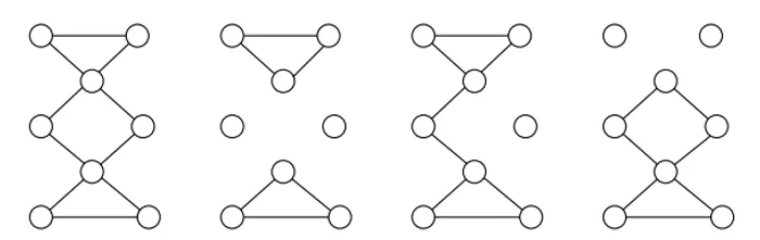
A generalized loop on $G$ is any subgraph $G(\tilde{E}) \subseteq G$ such for all $s \in G(\tilde{E})$ it holds $d_s(\tilde{E})\neq 1$

Given some stationary points of pseudomarginals after runnign message passing algorithm which minize the Bethe variational problem we obtain the following error expression w

$A(\theta)=A_{\mathrm{Bethe}}(\theta)+\log \Big\{ 1+\sum_{E \subseteq \tilde{E}}\beta_{\tilde{E}} \prod_{s\in V} \mathbb{E}_{\tau_{s}}[(X_{s}-\tau_{s})^{d_{s}(\tilde{E})}]\Big\}.$

where

$\beta_{s t}:=\,\frac{\tau_{s t}-\tau_{s}\tau_{t}}{\tau_{s}({\bf1}-\tau_{s})\tau_{t}({\bf1}-\tau_{t})}, \qquad \beta_{\tilde{E}}:=\prod_{(s,t)\in\tilde{E}}\beta_{s t}.$

denotes the edge weights associated to set of pseudomarginals $\xi$. In view of the above error bound we can make the following observations

• The error in the Bethe approximation is influenced by generalized loops in the graph, particularly those subgraphs $G(\tilde{E})$ where every vertex has a degree greater than one. The contribution of each loop to the error is weighted by $\beta_{\tilde{E}}$ which depends on the pseudomarginal estimates.
• For tree-structured graphs (where loops are absent), the error term vanishes, and the Bethe approximation becomes exact.

This result provides a systematic understanding of the accuracy of the Bethe entropy approximation and its dependence on the underlying graph structure.

Reparametrization Updates

Upper Bound on the Partition Function

Error Bounds