Weingarten Map

The measure of curvature at a point on a surface is an intrinsic property—it depends only on the distances on the surface and is independent of how the surface is embedded in space.
Carl Friedrich Gauss

Let $\mathcal{M}$ be an $m$ -dimensional submanifold in a $d$ -dimensional Euclidean space $\mathbb{E}^d$ with an induced Riemannian metric. At each point $p \in \mathcal{M}$ , consider the decomposition of the tangent space:

T_p \mathcal{M} \oplus T^{\perp}_p \mathcal{M} = \mathbb{E}^d.

For each normal vector $\xi \in T^{\perp}_p \mathcal{M}$ , let $\tilde{\xi}$ be the extension of $\xi$ to the whole manifold $\mathcal{M}$ . The Weingarten map or shape operator at $p \in \mathcal{M}$ with respect to $\xi$ is the mapping:

W_{\xi}(X) = -\Pi(\overline{\nabla}_X \tilde{\xi}),

where $\Pi: \mathbb{E}^d \to T_p \mathcal{M}$ is the orthogonal projection to the tangent space. An important property of the Weingarten map is that it is independent of the particular choice of extension $\tilde{\xi}$ .

Expanding the above map using a Taylor series yields:

Theorem

(\tilde{\xi}_{q} - \tilde{\xi}_{p})^{\top} = -A_{\tilde{\xi}_{p}}\left((q - p)^{\top}\right) + \mathcal{O}(\|q - p\|^{2}).

This makes it an attractive feature descriptor for measuring the variation of the normal vector field of a given dataset. We next illustrate how this is performed on an image data set and provide a guidelilne for an easy implementation in python.
Given an image $I$ , we first estimate the basis of the tangent and normal spaces at pixel $x_i$ by constructing the covariance matrix

\mathrm{C}_i = \sum_{j \in I_i} (x_{j} - \bar{x}_{i})(x_{j} - \bar{x}_{i})^{\dagger},

from which we can estimate a smooth normal vector field for each pixel $i \in x$ through through eigenvalue decomposition.

import numpy as np
from scipy.ndimage.filters import convolve

def Weingarten_Map(I,Mask_dim_x = 11,Mask_dim_y = 11):
        assert Mask_dim_x % 2 != 0 and Mask_dim_y % 2 != 0 
        Mask_dim_x = 11
        Mask_dim_y = 11
        N = (Mask_dim_x*Mask_dim_y)
        Mask = np.ones((Mask_dim_x,Mask_dim_y))/N

        Res_x = 1/I.shape[0]
        Res_y = 1/I.shape[1]


        Im_pred_vec = np.zeros((*I.shape,3))
        Im_pred_vec_mean = np.zeros((*I.shape,3))
        Im_pred_vec[:,:,2] = I[:,:]
        Im_pred_vec[:,:,0:2] = np.moveaxis(np.array(np.indices((Im_pred_vec.shape[0:2])),dtype = np.float32),0,-1)
        
        ' Add Resolution to the indices ' 
        
        Im_pred_vec[:,:,0:2] = np.einsum("ijk,k->ijk",Im_pred_vec[:,:,0:2],np.array([Res_x,Res_y]))
        Im_pred_vec_mean = convolve(Im_pred_vec,Mask[:,:,None])

        ' Compute Covariance Matrix '

        Im_pred_vec[:,:,0:2] = np.einsum("ijk,k->ijk",Im_pred_vec[:,:,0:2],np.array([Res_x,Res_y]))
        Im_pred_vec_mean = convolve(Im_pred_vec,Mask[:,:,None])
        Im_pred_vec_mean_w = convolve(Im_pred_vec,Mask[:,:,None])

        Cov_Mat = np.zeros((*I.shape,3,3))

        Cov_Mat =  N*convolve(np.einsum('ijk,ijl->ijkl', Im_pred_vec, Im_pred_vec), Mask[:, :, None,None], mode="nearest")
        Cov_Mat -= np.einsum('ijk,ijl->ijkl', Im_pred_vec_mean_w, Im_pred_vec_mean)
        Cov_Mat -= np.einsum('ijl,ijk->ijkl', Im_pred_vec_mean_w, Im_pred_vec_mean)
        Cov_Mat += np.einsum('ijk,ijl->ijkl', Im_pred_vec_mean, Im_pred_vec_mean)

The first $m$ largest eigenvectors of covariance matrix $C_i$ determine a basis for the tangent space approximation for each pixel location $i \in I$ . Hereby, the last $d-m$ eigenvectors determine a basis of corresponding normal space. Lets reproduce this part

'Compute normals and tangets for each pixel location'

N_space,T_space,_ = np.split(np.linalg.eigh(Cov_Mat)[1],(1,3),axis = 3)
N_space = np.squeeze(N_space)

To compute the Weingarten map, we need to extend the normal vector field smoothly across entire submanifold $\mathcal{M}$ . This is achieved by projecting $\xi_i$ to normal spaces at each pixel $j \in I$ which results in a smooth normal vector field

\tilde{\xi}_{x_j}^{\alpha} = \sum_{\beta=1}^{d-m} \langle \xi_{i}^{\alpha}, \xi_{j}^{\beta} \rangle \xi_{j}^{\beta}.

Consider a twice-differentiable function supported on the interval $[0, 1]$ and a parameter $h > 0$ which defines a scaled kernel:

K_{h}(y) = \frac{1}{h^{m}} K\left(\frac{\|y\|}{h}\right).

Leveraging the tangent basis $E_i$ at pixel $i$ and assuming that $x_i$ is close to $x_j$ , the Result simplifies to the following first-order approximation of the Weingarten map:

(\tilde{\xi}_{x_j}^{\alpha} - \xi_{i}^{\alpha})^{\top} \mathcal{E}_{i} = -(x_j - x_i)^{\top} \mathcal{E}_{i} A_{\xi_{i}}^{\alpha} + \mathcal{O}(\|x_j - x_i\|^{2}),

where $A_{\xi_i^{\alpha}} \in \mathbb{R}^{m \times m}$ . As a consequence, in order to get access to the Weingarten map need to minimize the objective

\sum_{j=1}^{n} \|\left(\tilde{\xi}_{x_j}^{\alpha} + \xi_{i}^{\alpha}\right)^{\dagger} \mathcal{E}_{i} - (x_j - x_i)^{\dagger} \mathcal{E}_{i} \tilde{A_{\xi^{\alpha}_i}}_{\tilde{i}} \|^{2} \mathcal{K}_{h}(x_j - x_i), \qquad (1)

Introducing the auxiliary mappings:

\begin{array}{l}\widetilde{\Delta}_{i} = E_{i}^{\dagger} \left[x_{1} - x_{i}, \ldots, x_{n} - x_{i}\right],\\ \widetilde{\Xi}_{i}^{\alpha} = E_{i}^{\dagger} \left[\widetilde{\xi}_{x_1}^{\alpha} - \xi_{i}^{\alpha}, \ldots, \widetilde{\xi}_{x_n}^{\alpha} - \xi_{i}^{\alpha}\right], \\ \mathcal{M}_{i} = \mathrm{diag} \{ K_{h}(x_1 - x_i), \ldots, K_{h}(x_n - x_i) \}.\end{array}\qquad (2)

solution to optimization problem (1) exhibits a closed-form solution such that the Weingarten map at each pixel $i\in I$ is represented in terms of the decomposition

\widetilde{A}_{\xi_i^{\alpha}} = -\widetilde{\Xi}_{i}^{\alpha} W_{i} \widetilde{\Delta}_{i}^{\dagger} (\widetilde{\Delta}_{i} W_{i} \widetilde{\Delta}_{i}^{\dagger})^{-1}.\qquad (3)

Note, that we need to compute $(2)$ for all pixels $i \in I$ which involves the sum over all pixel to evaluate the objective (1).
This results in large dimension of matrices in (2). Due to the exponential decay of the kernel function we instead use an approximation by summing over a suffieciently large neighbourhood.

N_space_pad = np.pad(N_space,((X_shift-1,X_shift-1),(Y_shift-1,Y_shift-1),(0,0)))
N_space_pad = view_as_windows(N_space_pad,(Mask_dim_x,Mask_dim_y,3),step=(1, 1, 1))
N_space_pad =  np.squeeze(N_space_pad)
Delta_k = np.einsum('ijlk,ijsml->ijsmk',T_space[:,:,:,:],X_diff)
Scalar_Mat = np.einsum('ijsmk,ijk->ijsm',N_space_pad,N_space)
N_space_pad = N_space_pad*Scalar_Mat[:,:,:,:,None]-N_space[:,:,None,None,:]
Theta_k = np.einsum('ijkl,ijsmk->ijsml',T_space,N_space_pad)
Diag_W = np.exp(-np.einsum('ijkls,ijkls->ijkl',X_diff,X_diff)/(sigma**2))/(sigma**2)
W_Matrix = -np.einsum('ijsmk,ijsml->ijkl',Theta_k*Diag_W[:,:,:,:,None],Delta_k)
Theta_k = np.einsum('ijsmk,ijsml->ijkl',Delta_k*Diag_W[:,:,:,:,None],Delta_k)+0.1*np.eye(2)[None,None,:,:]
Theta_k = np.linalg.inv(Theta_k.reshape(-1,2,2)).reshape(*Theta_k.shape)
W_Matrix = np.einsum('ijsk,ijkm->ijsm',W_Matrix,Theta_k)
W_Matrix = 0.5*(W_Matrix+np.swapaxes(W_Matrix,axis1=2,axis2=3))

Given the Weingarten map, we gain access to the second fundamental form, mean curvature, and sectional curvature at each image location $i$ . These features can be used for classification and segmentation tasks.

Gauss Formuala and the Second Fundamental Form

For each submanifold $\mathcal{M} \subset \mathcal{N}$ with the corresponding induced Riemannian metric we denote by $\overline{\nabla}$ the connection on $\mathcal{N}$ and $\nabla$ the connection on $\mathcal{M}$ . Then for any pair of vector fields $X,Y \in \mathcal{X}(M)$ we have the Gauss formula.

\overline{{{\nabla}}}_{X}Y=\nabla_{X}Y+h(X,Y) \qquad \nabla_{X}Y=\left(\overline{{{\nabla}}}_{X}Y\right)^{\top},h(X,Y)=\left(\overline{{{\nabla}}}_{X}Y\right)^{\perp}

the map $h:\mathcal{X}(M) \times \mathcal{X}(M) \to \Gamma(T^{\perp}\mathcal{M})$ is a second-order symmetric covariant tensor field on $\mathcal{M}$ commonly known as the second fundamental form of submanifold $\mathcal{M}$ . For each normal vector field $\xi$ the second fundamental form and the Weingarten are related by the Weingarten formula

\overline{\nabla}_{X}\xi = -A_{\xi}(X)+\nabla_X^{\perp}\xi

with

A_{\xi}(X) = (\overline{\nabla}^{\perp}_X\xi)^T, \qquad \nabla^{\perp}_X\xi = (\overline{\nabla}_X\xi)^{\perp}

The following plot illustrates the computed curvature measurues that can be used for a feature extraction filter bank

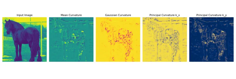
Curvature

The Weingarten Map $W$ is a $2 \times 2$ symmetric matrix that encodes the curvature information of a surface. Using $W$ , we can define the following curvatures:

Principal Curvatures

The principal curvatures $\kappa_1$ and $\kappa_2$ are the eigenvalues of $W$ , given by:

$\kappa_{1,2} = \frac{\text{tr}(W) \pm \sqrt{\text{tr}(W)^2 - 4 \, \text{det}(W)}}{2}$

where:

$\text{tr}(W)$ is the trace of $W$ ( $w_{11} + w_{22}$ ).
$\text{det}(W)$ is the determinant of $W$ ( $w_{11}w_{22} - w_{12}^2$ ).

Mean Curvature

The mean curvature $H$ is the average of the principal curvatures:

$H = \frac{\kappa_1 + \kappa_2}{2} = \frac{\text{tr}(W)}{2}$

Gaussian Curvature

The Gaussian curvature $K$ is the product of the principal curvatures:

$K = \kappa_1 \cdot \kappa_2 = \text{det}(W)$

nx,ny = W_Matrix.shape[0:2]
mean_curvature = np.zeros((nx, ny))
gaussian_curvature = np.zeros((nx, ny))
principal_curvatures = np.zeros((nx, ny, 2))  # Store kappa1, kappa2

# Compute eigenvalues and curvatures
for i in range(nx):
    for j in range(ny):
        W = W_Matrix[i, j]
        # Compute eigenvalues (principal curvatures)
        kappa1, kappa2 = np.linalg.eigvalsh(W)  # Use eigvalsh for symmetric matrices
        principal_curvatures[i, j] = [kappa1, kappa2]
        # Mean and Gaussian curvatures
        mean_curvature[i, j] = 0.5*(kappa1 + kappa2)
        gaussian_curvature[i, j] = kappa1 * kappa2