Expectation Maximization (EM)

A widely applied parametric counterpart to soft-k-means clustering for acquiring prototypes on a measurable space $\mathcal{X}$ is based on the assumption of i.i.d. random samples $x_i \in X_n$ and by the following parametric family of mixture distributions:

$p(x,\Gamma) = \sum \limits_{j\in [k]} \pi_jp(x,\theta_j)\qquad \Gamma = (\theta,\pi),$

with unknown parameters:

$\Gamma = (\theta,\pi), \qquad \theta = (\theta_1,\dots,\theta_k) \qquad \pi = (\pi_1,\dots,\pi_k)^T \in \Delta_k.$

Here, the different parameters $\theta_j \in \Theta, j \in [k]$ parameterize the mixture distribution on $\mathcal{X}$ that partitions the set $\mathcal{X}_n$ into $k$ different clusters with proportions $\pi \in \mathcal{S}$, where each $x_i$ has the density $p(x_i,\theta_j)$.

Starting from this statistical perspective, where an approximation $\hat{\Gamma} = (\hat{\theta},\hat{\Gamma})$ to model parameters $\Gamma$ is given, clustering amounts to fitting the mixture distribution $p(x, \Gamma)$ by estimating true model parameters $\Gamma$ via maximum log-likelihood estimation of:

$L(\theta) = \sum \limits_{i \in [n]}\log \big(\sum \limits_{j \in [k]} \pi_j p(x_i,\theta_j) \big).$

Making a further assumption that each $x_i$ is generated by exactly one component distribution $p(j,\Gamma)$ and augmenting the set:

$(\mathcal{X}_n,\mathcal{Y}_n) = (x_1,\dots,x_n,y_1,\dots y_n), \qquad x_i \in \mathcal{X}_n, y_i \in [k]$

where $y_i$ corresponds to class assignments of points $x_i$ to the associated distribution $p(x_i,\theta_{y_i})$, optimization is performed by instead maximizing the following lower bound to $L(\theta)$:

$\sum_{j \in [k]}\sum_{i \in [n]}p(j|x_i,\hat{\Gamma})\log\left(\frac{p(x_i,j,\Gamma)}{p(j|x_i,\hat{\Gamma})}\right).$

Maximization of this lower bound amounts to performing the so-called EM-iterates (expectation-maximization), see [Bishop, 2007], that result in the updates with initialization $\Gamma^{(0)} = \hat{\Gamma}$:

$\Gamma^{(t)}(\theta^{(t)},\pi^{(t)}).$

EM Algorithm Updates:

1. Expectation Step:

   $p(j|x_i,\Gamma^{(t)}) = \frac{\pi_j^{(t)}p(x_i,\Gamma^{(t)})}{\sum_{l \in [k]}\pi_l^{(t)}p(x_i,\Gamma^{(t)})}$

2. Maximization Step for $\pi$ and $\theta$:

   $\pi_j^{(t+1)} = \frac{1}{n}\sum \limits_{i \in [n]}p(j|x_i, \Gamma^{(t)}),$

   $\theta^{(t+1)} = \arg\max \limits_{\theta_j}\sum \limits_{i \in [n]} p(j|x_i,\Gamma^{(t)})\log p(x_i,\theta_j).$

The procedure consists of two main steps: $(i)$ expectation over the conditional distributions $p(j|x_i,\hat{\Gamma})$ yielding a lower bound for the objective $L(\theta)$, and $(ii)$ maximization over parameter $\theta$.

Exponential Family Distribution Case:

For the case where the components $p(x,\theta_j)$ belong to an exponential family of distributions represented in terms of Bregman divergence:

$p(x,\Gamma) = \sum_{j \in [k]} \pi_j \exp(-D_{f}(F(x),\nu_j))b_f(x),$

where parameters are expressed via conjugation through:

$\Gamma = (\nu,\pi), \qquad \nu = (\nu_1,\dots,\nu_k) \quad \text{with} \quad \nu_j = \psi(\theta_j), \quad j \in [k].$

The EM updates simplify to:

1. Expectation Step with Bregman Divergence:

   $p(j|x_i,\Gamma^{(t)}) = \frac{\pi_j^{(t)}\exp(-D_f(F(x_i),\psi(\theta_j^{(t)})))}{\sum_{l \in [k]}\pi_l^{(t)}\exp(-D_f(F(x_i),\psi(\theta^{(t)}_l)))}$

2. Maximization Step:

   $\pi_j^{(t+1)} = \frac{1}{n}\sum \limits_{i \in [n]}p(j|x_i, \Gamma^{(t)}),$

   $\nu^{(t)}_{ij} = \frac{p(j|x_i,\Gamma^{(t)})}{\sum_{s \in [n] }p(j|x_s,\Gamma^{(t)})},$

   $\mu_j^{(t+1)} = \arg\min \limits_{\mu_j}\sum_{i \in [n]}\nu^{(t)}_{ij} D_f(F(x_i),\mu_j),$

where the final step admits a closed-form solution similar to mean shift updates:

$\mu_j^{(t)} = \sum_{i \in [n]} \nu_{ij}^{(t)}F(x_i).$

For detailed treatment of EM iterates in connection with Bregman divergences, see [Banerjee, 2005].

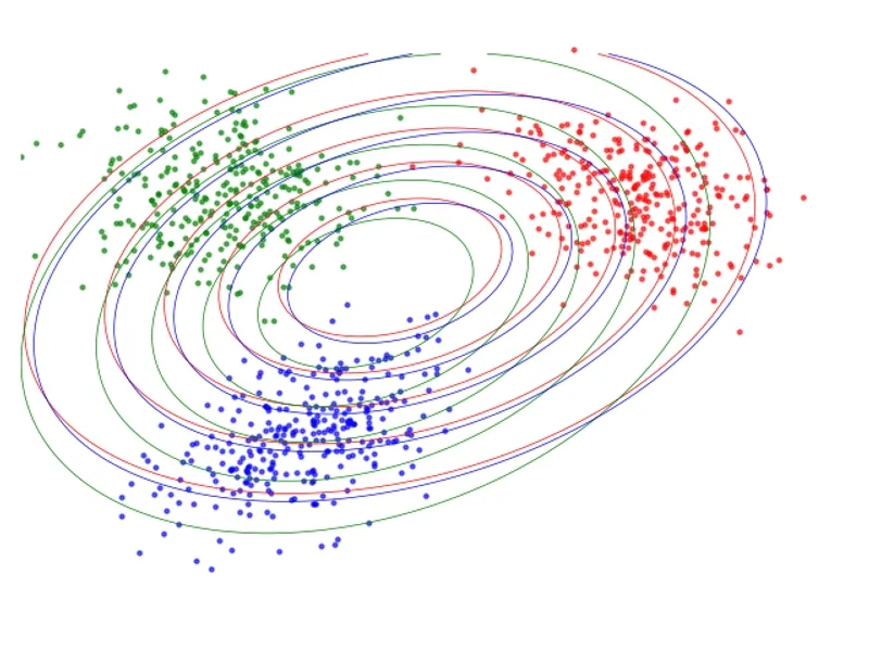
Lets consider a simple example of applying the EM algorithm to fitting a mixture of 3 gaussions. Given a data set $\mathcal{D}$ generated from $p(x,\mu_i,\Sigma_i)$ with

$\mu_1 = \begin{pmatrix} 1.9 \\ 2.1 \end{pmatrix}, \quad \mu_2 = \begin{pmatrix} 6.8 \\ 7.1 \end{pmatrix}, \quad \mu_3 = \begin{pmatrix} 1.2 \\ 6.9 \end{pmatrix} \quad \\\\\ \Sigma_1 = \begin{pmatrix} 0.95 & 0.45 \\ 0.45 & 1.05 \end{pmatrix}, \quad \Sigma_2 = \begin{pmatrix} 1.1 & -0.25 \\ -0.25 & 1.0 \end{pmatrix}, \quad \Sigma_3 = \begin{pmatrix} 1.0 & 0.0 \\ 0.0 & 1.1 \end{pmatrix}$