Exact Marginal Estimation via Junction Trees

Junction trees, also known as clique trees comprises a particular type of data structure used in probabilistic graphical models for the inference of exact marginals of a given joint probability distribution.

We start with a simple graphical model constisting of four nodes that form tree.

Knowing the joint distribution $p(x_1,x_2,x_3,x_4)$ our goal are the marginals $p(x_1),p(x_2),p(x_3),p(x_4)$. A simple apporach is the marginalization over the complementary set, i.e. for $x_3$

$\begin{aligned} \sum_{x_1,x_2,x_4} p(x_1,\dots,x_4) = p(x_3) \end{aligned}$

which requires $10^3$ summations if we assume $x_i$ to be a categorical random variable taking values in the finite set $\{1,\dots 10\}$. However, for larger graphs this procedure scales exponential with the number of nodes $|V| = n$ in the graph resulting in $10^{90}$ summations for each marginal which is more then the number of atoms in the universe! A way out of this hopeless apporach is given by the underlying tree structure of the graph with respect to which the disribution can be rewritten as

$\begin{aligned} p(x_1,x_2,x_3,x_4) &= \frac{p(x_1,x_2,x_3,x_4)p(x_3,x_2,x_1)}{p(x_3,x_2,x_1)}\\ &= p(x_4|x_3,x_2,x_1)p(x_3,x_2,x_1)\\ &=p(x_4|x_3,x_2,x_1)p(x_2|x_3,x_1)p(x_1,x_3)\\ &= p(x_4|x_3,x_2,x_1)p(x_2|x_3,x_1)p(x_1,x_3)p(x_1|x_3)p(x_3) \end{aligned}$

As the node $x_3$ separates the connecting nodes $x_1,x_2$ and $x_4$ and therefore by conditional independence using $p(x_4|x_3,x_2,x_1) = p(x_4|x_3)$ and $p(x_2|x_3,x_1) = p(x_2|x_3)$ the joint probability distribution factorizes into the product of conditional distributions

$\begin{aligned} p(x_1,x_2,x_3,x_4) &= p(x_1,x_2,x_4|x_3)p(x_3) \\&= p(x_1|x_3)p(x_2|x_3)p(x_4|x_3)p(x_3)\\ &= \frac{p(x_1,x_3)p(x_2,x_3)p(x_4,x_3)}{p(x_3^2)} \end{aligned}$

So far nothing is won, because taking off from the right hand side we still have to sum over nodes $\{x_1,x_2,x_4\}$. However, if we would have knowledge on the edge marginals $p(x_i,x_3)$, we could reselve this problem by just taking the sum over $x_i$. This is the essence why estimating the marginals of a large joint probability distribution concerns so much attention in the scientific communnity.

Following the steps we have now reduced the marginalization problem to inference task of edge marginals. But how do we arrive at the right hand side if we have more complecated graphs ? Before answering this quastion we state an alternative factorization of $p(x)$

$\begin{aligned} \frac{p(x_1,x_3)p(x_2,x_3)p(x_4,x_3)}{p(x_3^2)} = \frac{p(x_1,x_3)}{\textcolor{red}{p(x_1)}p(x_3)}\cdot \frac{p(x_2,x_3)}{p(x_3)\textcolor{red}{p(x_2)}}\cdot\frac{p(x_4,x_3)}{\textcolor{red}{p(x_4)p(x_3)}}\cdot\textcolor{red}{p(x_3)p(x_1)p(x_2)p(x_4)} \end{aligned}$

Now even if we dont have acces to true marginals $p(x_i,x_k)$ we still have the global distribution from the left and factorization from the right which we can use to model our distribution

$\begin{aligned} p(\bold{x}) = \psi_1(x_1)\psi_2(x_2)\psi_3(x_3)\psi_4(x_4)\psi_{13}(x_1,x_3)\psi_{23}(x_2,x_3)\psi_{34}(x_3,x_4) \end{aligned}$

which agrees with the previous factorization for the particular case $\psi_i(x_i) = p(x_i)$ and $\psi_{ij}(x_i,x_j) = \frac{p(x_i,x_j)}{p(x_i)p(x_j)}$. Now given any factorization with respect to potential functions $\psi_{ij}(x_i,x_j)$ how can we effiently acces the marginal at $p(x_1)$? To get an intuition we consider a simple scenario of a chain consisting of three nodes $x_1,x_2$ and $x_3$

$\begin{aligned} p(x_1,x_2,x_3) \propto \tilde{\psi}^{(0)}_1(x_1)\tilde{\psi}^{(0)}_3(x_3)\psi^{(0)}_4(x_4)\tilde{\psi}^{(0)}_{13}(x_1,x_3)\tilde{\psi}^{(0)}_{34}(x_3,x_4) = \frac{\psi^{(0)}_{13}(x_1,x_3)\psi^{(0)}_{13}(x_3,x_4)}{\psi_3^{(0)}(x_3)}, \qquad \psi_3^{(0)}(x_3) = 1 \end{aligned}$

We want the updates of local potentials $\psi^{(n)}(x_1,x_3)\psi^{(n)}_{3}(x_3)$ and $\psi^{(n)}(x_1,x_3)\psi^{(n)}_{3}(x_3)$ that in the limits satisfy a constaint

$\begin{aligned} \sum_{x_1}\frac{p(x_1,x_3)}{p(x_3)} = \sum_{x_4}\frac{p(x_3,x_4)}{p(x_3)} = 1 \end{aligned}$

Now assume that this local consistancy condition is not satisfied , that is

$\begin{aligned} \sum_{x_1}\psi^{(0)}_{13}(x_1,x_3) \neq \sum_{x_4}\psi^{(0)}_{34}(x_3,x_4) \end{aligned}$

at the next iteration we want fix this by first updating the separator node marginal $\psi^{(1)}_{3}(x_3) = \sum_{x_1} \psi^{(0)}_{13}(x_1,x_3)$

and then normalize the edge potential

$\psi^{(1)}_{34}(x_3,\cdot) = \frac{\psi^{(1)}_3(x_3)\psi^{(0)}_{34}(x_3,\cdot)}{\psi_3^{(0)}(x_3)}$

For the above steps to be admissible two aspect must hold

$(i)$: The factorization with respect does not effect the joint probability, i.e.

$\begin{aligned} \frac{\psi^{(0)}_{13}(x_1,x_3)\psi^{(1)}_{34}(x_3,x_4)}{\psi_3^{(1)}(x_3)} = \frac{\psi^{(0)}(x_1,x_3)\psi_3^{(1)}(x_3)\psi^{(0)}_{34}(x_3,x_4)}{\psi_3^{(0)}(x_3)\psi_3^{(1)}(x_3)} = p(x_1,x_3,x_4) \end{aligned}$

$(ii)$: the local consistancy condition at $x_3$:

$\begin{aligned} \sum_{x_1}\psi^{(0)}_{13}(x_1,x_3) = \psi^{(1)}_{3}(x_3) \neq \sum_{x_4}\psi^{(1)}_{34}(x_3,x_4) = \sum_{x_4}\frac{\psi^{(1)}_{3}(x_3)\psi^{(0)}_{34}(x_3,x_4)}{\psi^{(0)}_3(x_3)} \end{aligned}$

which is still violated due to $\psi^{(0)}_3(x_3) = 1 \neq \sum_{x_4}\psi^{(0)}_{34}(x_3,x_4)$ by assumption. However, what we have achieved is $(iii)$: marginalization condition at the edge $(34)$ as

$\begin{aligned} \psi_{34}^{(1)}(x_3,x_4) = \sum_{x_1}\underbrace{\frac{\psi^{0}_{13}(x_1,x_3)\psi^{(0)}_{34}(x_3,x_4)}{\psi_3^{(0)}(x_3)}}_{= p(x_1,x_2,x_3)} = p(x_3,x_4) \end{aligned}$

This process of propagating the marginal from leaf node $x_1$ over separator node $x_3$ over to leaf node $x_4$ is commonly denoted as the forward pass which leads the true marginal distribution $\psi^{\ast}(x_3,x_4)$. Now by contruction we can do the same in the reverse direction by repeating the steps

• $\psi_3^{(2)}(x_3) = \sum_{x_4}\psi^{\ast}_{34}(x_3,x_4)$

and then updating the edge potential

$\begin{aligned} \psi^{(\ast)}_{13}(x_1,x_3) = \frac{\psi_3^{(2)}(x_3)\psi_{13}^{(0)}(x_1,x_3)}{\psi_3^{(1)}(x_3)} \end{aligned}$

which defines the backward pass

and we next check again the three conditions

$\bullet$ Joint probability distribution:

$\begin{aligned} \frac{\textcolor{green}{\psi^{\ast}_{13}(x_1,x_3)}\textcolor{red}{\psi^{\ast}_{34}(x_3,x_4)}}{\psi^{(2)}_3(x_3)} &= \frac{\textcolor{green}{\psi_3^{(2)}(x_3)\psi^{(0)}_{13}(x_1,x_3)}\textcolor{red}{\psi^{(1)}_{34}(x_3,x_4)}}{\textcolor{green}{\psi_3^{(1)}(x_3)}\psi_3^{(2)}(x_3)}\\ &=\frac{\textcolor{green}{\psi^{(0)}_{13}(x_1,x_3)}\textcolor{red}{\psi^{(1)}_{3}(x_3)\psi^{(0)}_{34}(x_3,x_4)}}{\textcolor{green}{\textcolor{red}{\psi^{(0)}_3(x_3)}\psi_3^{(1)}(x_3)}}\\ &=\frac{\textcolor{green}{\psi^{(0)}_{13}(x_1,x_3)}\textcolor{red}{\psi^{(0)}_{34}(x_3,x_4)}}{\textcolor{green}{\psi_3^{(0)}(x_3)}}\\ &=p(x_1,x_2,x_3) \end{aligned}$

$\bullet$ Local consistancy:

$\begin{aligned} \sum_{x_1}\psi_{13}^{\ast}(x_1,x_3) &= \frac{\psi^{(2)}_3(x_3)}{\psi_3^{(1)}(x_3)}\sum_{x_1}\psi^{(0)}_{13}(x_1,x_3)\\ &= \frac{\psi^{(2)}_3(x_3)}{\psi_3^{(1)}(x_3)}\underbrace{\sum_{x_1}\psi^{(0)}_{13}(x_1,x_3)}_{\psi_3^{(1)}(x_3)}\\ &= \sum_{x_4}\psi^{(1)}_{34}(x_3,x_4) \end{aligned}$

$\bullet$ Correct edge marginals:

$\begin{aligned} \psi^{\ast}_{13}(x_1,x_3) &= \frac{\psi^{(2)}_{3}(x_3)\psi^{(0)}_{13}(x_1,x_3)}{\psi^{(1)}_{3}(x_3)}\\ &= \frac{\sum_{x_4}\psi_{34}^{(\ast)}(x_3,x_4)\psi^{(0)}_{13}(x_1,x_3)}{\psi^{(1)}_{3}(x_3)} &=\sum_{x_4} \underbrace{\frac{\psi_3^{(1)}(x_3)\psi_{34}^{(0)}(x_3,x_4)\psi^{(0)}_{13}(x_1,x_3)}{\psi^{(1)}_{3}(x_3)\psi_3^{(0)}(x_3)}}_{= p(x_1,x_3,x_4)} &= p(x_1,x_3) \end{aligned}$

and consequently we obtain a new factorization of the joint probabilty with

$\begin{aligned}\psi^{\ast}_{13}(x_1,x_3) = p(x_1,x_3),\quad \psi^{\ast}_{34}(x_3,x_4) = p(x_3,x_4) \quad \psi^{\ast}_3(x_3) = p(x_3)\end{aligned}$

We can generalize the above procedure from chain graph to simple tree graph by including node $x_2$ adding the missing compenents in the factorization of $\psi_{34}^{(1)}(x_3,x_4)$ in the forward pass to yield correct edge potential $p(x_3,x_4)$ via additional marginalization over new node $x_2$.

$\begin{aligned} \psi_{34}^{(1)}(x_3,x_4) &= \sum_{x_1}\textcolor{red}{\sum_{x_2}} \frac{\psi^{0}_{13}(x_1,x_3)\psi^{(0)}_{34}(x_3,x_4)\textcolor{red}{\psi^{0}_{23}(x_2,x_3)}}{\psi_3^{(0)}(x_3)\textcolor{red}{\psi_3^{(0)}(x_3)}}\\ &= \frac{\textcolor{red}{\psi^{(1)}_{1\to 3}(x_3)} \textcolor{red}{\psi^{(1)}_{2 \to 3}(x_3)}\psi^{(0)}_{34}(x_3,x_4)}{\psi_3^{(0)}(x_3)^{2}}\\ &= \sum_{\textcolor{red}{x_2},x_1} p(x_1,\textcolor{red}{x_2},x_3,x_4) = p(x_3,x_4) \end{aligned}$

Simply put we the above update corresponds to a simple forward pass where now we have a set of messages $\psi^{(1)}_{i \to 3}(x_3)$ coming through a separating node $x_3$ from from edges connected to it. The of message passing updates now comes from the fact that we can interpret the current marginals at $x_3$ as messages from marginalized node over $x_3$ over to leaf node $x_4$. Now repeating the steps of the backward pass but now with additional edge potential $\psi_{23}^{(\ast)}(x_2,x_3)$ it follows

$\begin{aligned} \psi^{\ast}_{23}(x_2,x_3) &= \frac{\psi^{(2)}_{4 \to 3}(x_3)\psi^{(0)}_{23}(x_2,x_3)}{\psi^{(1)}_{2 \to 3}(x_3)}\\ &= \frac{\sum_{x_4}\psi_{34}^{(\ast)}(x_3,x_4)\psi^{(0)}_{23}(x_2,x_3)}{\psi^{(1)}_{2 \to 3}(x_3)} \\ &=\sum_{x_4}\sum_{x_1} \frac{\psi_{2 \to 3}^{(1)}(x_3)\psi_{13}^{(0)}(x_1,x_3)\psi_{34}^{(0)}(x_3,x_4)\psi^{(0)}_{23}(x_2,x_3)}{\psi^{(1)}_{2 \to 3}(x_3)(\psi_3^{(0)}(x_3))^2}\\ &= \sum_{x_1,x_4}p(x_1,x_2,x_3,x_4) = \ p(x_2,x_3) \end{aligned}$

It can easely be checked that all condition hold and we get the correct marginals from the backward pass. The following graphic illustrates the steps

More generally on a tree graph with node size $|V| = n$ each tree-structured distribution factorizes via local marginals

$\begin{aligned} p(\bold{x}) = \prod_{i \in V}p(x_i)\prod_{(x_i,x_j) \in E}\frac{p(x_i,x_j)}{p(x_i)p(x_j)} \qquad \bold{x} = (x_1,\dots,x_n) \end{aligned}$

where:

• $p(x_i)$ are the marginal probability at node $v \ in V$ on a tree graph $\mathcal{G}^T = (V,E)$,
• $p(x_i, x_j)$ are the pairwise joint probabilities on edges $(i, j) \in E$,
• The fraction $\frac{p(x_i, x_j)}{p(x_i) p(x_j)}$ is now the desired representation of $\psi_{ij}(x_i,x_j)$ in terms of marginals.

This can be seen as follows

First, each node $x_i$ on a tree is conditionally independent of all other nodes given its neighbors, i.e. the joint distribution satisfies the pairwise Markov property:

$p(x_i \mid x_{V \setminus \{i\}}) = p(x_i \mid x_{\text{neigh}(i)})$

where $\text{neigh}(i)$ is the set of neighboring nodes of $i$. The joint distribution can be expanded using the chain rule for probabilities

$p(x_1, x_2, \dots, x_n) = \prod_{i \in V} p(x_i \mid x_{j < i}) = \prod_{i \in V} p(x_i \mid x_{\text{parents}(i)})$

where $\text{parents}(i)$ refers to the parent of vertex $i$ with respect to some arbitrary root of the tree.

Second, for each vertex $i \in V$, its conditional distribution $p(x_i \mid x_{\text{parents}(v)})$ can be expressed using the joint marginal $P(X_v, X_{\text{parents}(v)})$ and the marginal $P(X_{\text{parents}(v)})$ via

$p(x_i \mid x_{\text{parents}(i)}) = \frac{P(x_i, x_{\text{parents}(i)})}{p(x_{\text{parents}(i)})}$

which after insertion into the joint probability yields the desired factorization

$p(x_1, x_2, \dots, x_n) = \prod_{(i, j) \in E} \frac{p(x_i, x_j)}{p(x_i)} = \prod_{i \in V}p(x_i) \prod_{(i,j)\in E}\frac{p(x_i, x_j)}{p(x_i)p(x_j)}$

where the last equality can be shown using induction over $n = |V|$.

As next more sophisticated example we consider the following graphical model with cycles on the $9\times 9$ ineteger grid

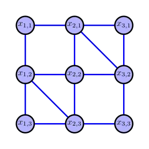
with an underlying distribution $p(x_1,\dots,x_9)$. We want to go for the marginals $p(x_1),p(x_3),p(x_7),p(x_9)$. A naive approach what we can do, say for accessing $p(x_7)$ is taking a sum over all nodes $x_k$ except $x_7$ which results in

$\begin{aligned} \sum_{x_{k\setminus 7}}p(x) = p(x_7) \end{aligned}$

which scales exponentially as $\mathcal{O}(8^r)$ with the node dimension $r$. However we can follow the same idea and determine $p(x_7)$ by performing message passing on a tree graph. However, due to presence of cycles we introduce a slight generalization of tree graph the so called junction trees.

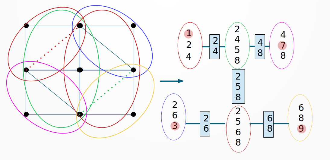
A junctio tree, consists of maximal cliques (subsets of fully connected nodes) of an triangulated graph, i.e. a graph with cycles of maximal length 3. The edges are defined in terms of the separater sets, i.e. intersection of adjacent cliques. In addition, the tree must satisfy the running intersection property, that is for each two maximal cliques $\mathcal{C}_1,\mathcal{C}_2$ and a node $x_j \in mathcal{C}_1 \cap mathcal{C}_2$ all cliques $\mathcal{C}_k$ and separater nodes $S_k$ on the path between $\mathcal{C}_1$ and $\mathcal{C}_2$ include $x_j$ The following figure illustrates a valid junctio tree for the above grid graph.

#include <iostream>
#include <vector>
#include <unordered_set>

using namespace std;

struct Node {
    int id;
    vector<int> neighbors;
};

struct Clique {
    unordered_set<int> nodes;
};

class Graph {
    int V;
    vector<Node> nodes;

public:
    Graph(int V);
    void addEdge(int v, int w);
    vector<Clique> triangulate();
    void printJunctionTree(const vector<Clique>& cliques);
};

Graph::Graph(int V) {
    this->V = V;
    nodes.resize(V);
    for (int i = 0; i < V; ++i) {
        nodes[i].id = i;
    }
}

void Graph::addEdge(int v, int w) {
    nodes[v].neighbors.push_back(w);
    nodes[w].neighbors.push_back(v);
}

// Triangulation using minimum fill-in heuristic
vector<Clique> Graph::triangulate() {
    vector<Clique> cliques;

    // Temporary vector to store the triangulated nodes
    vector<bool> processed(V, false);

    for (int i = 0; i < V; ++i) {
        if (!processed[i]) {
            // Find the neighbors of current node
            unordered_set<int> neighbors(nodes[i].neighbors.begin(), nodes[i].neighbors.end());

            // Add the node and its neighbors to a new clique
            Clique clique;
            clique.nodes.insert(i);
            for (int neighbor : nodes[i].neighbors) {
                clique.nodes.insert(neighbor);
                for (int n : nodes[neighbor].neighbors) {
                    if (n != i)
                        clique.nodes.insert(n);
                }
            }

            // Add the new clique to the junction tree
            cliques.push_back(clique);

            // Mark all nodes in the new clique as processed
            for (int node : clique.nodes)
                processed[node] = true;
        }
    }

    return cliques;
}

void Graph::printJunctionTree(const vector<Clique>& cliques) {
    cout << "Junction Tree:" << endl;
    for (int i = 0; i < cliques.size(); ++i) {
        cout << "Clique " << i << ": ";
        for (int node : cliques[i].nodes) {
            cout << node << " ";
        }
        cout << endl;
    }
}

int main() {
    Graph graph(6);
    graph.addEdge(0, 1);
    graph.addEdge(0, 2);
    graph.addEdge(1, 2);
    graph.addEdge(1, 3);
    graph.addEdge(2, 4);
    graph.addEdge(3, 4);
    graph.addEdge(3, 5);
    graph.addEdge(4, 5);

    vector<Clique> cliques = graph.triangulate();
    graph.printJunctionTree(cliques);

    return 0;
}