Variational Auto-Encoders (VAEs)

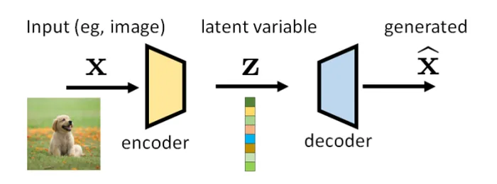
Vartiational Autoencoders become popular with the work of Kingma and Welling (2013). The primary goal was the inference task of latent distribution $p_{\theta}(z)$
over small instrictic dimension $\dim(z)$ thereby reducing the large dimensialel data space $\dim X$.

Chalenges:

• Evaluating the model evidence $p_{\theta}(x) = \int_Z p_{\theta}(x,z)dz$ is a hard task due to the involved integral. As $p_{\theta}(x,z)$ can be easy evaluated this implies that the conditional distribution $p_{\theta}(z|x) = \frac{p_{\theta}(x,z)}{p_{\theta}(x)}$ can not be accessed.

Variational Autoencoders assumes builds upon two variational distributions $p_{\theta}(x,z)$ and $p_{\phi}(x,z)$ which conditioned on the input random variable are denoted as the decoder and the encoder respectivaly.
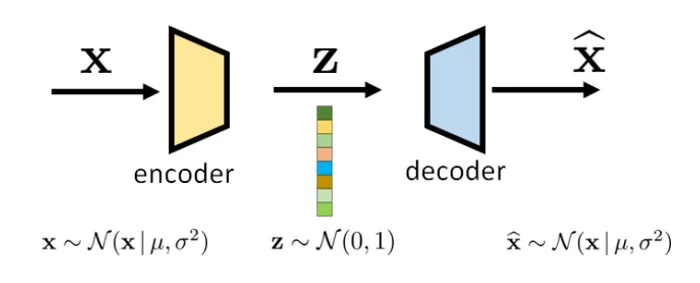
Hereby, common choices of the decoder $p_{\theta}(z|x)$ and the encoder $q_{\phi}(z|x) = \mathcal{N}(z;\phi)$ are assumed to be gaussian distribution whose mean and covariances are the deep paramterized by an neural network.

Evidence Lower Bound

The lower bound to the log-likelihood after skipping the nonnegative Kullback Leibner divergence is denoted as the Evidence-Lower-Bound Objective (ELBO). Therefore by maximizing the (ELBO) we follow the hope that corresponding maximimzer $\theta^{\ast},\mu^{\ast}$ of the Encoder Decoder part yield a maximmal log probability distribution $p_{\theta}(x)$.
Lets summerize our goal which potentially aim to achieve to get an optimal variational auto encoder:

• (1) We want an approximation to the truth data generating distribution,

which also highlights the burden to evaluate the conditional distribution over the latent space corresponding to the decoder $p_{\theta}(z|x)$ which by Bayes rule requires knowledge on $p^{\ast}(x)$ which is unknown.

by marginalizationg of the decoder.

• (2) By contruction the encoder $q_{\phi}(x,z)$ and the decoder $p_{\theta}(x,z)$ must satisfy the self-consitancy relation at the latent marginals $z\in Z$, i.e.

The distribution $q(z)$ over the latent space is commonly chosen to be a simple distribution to allow efficient sampling from the decoder $p_{\theta}(x|z)$ under assumption on tractable form of $p_{\theta}(x,z)$

• (3) Zero gap which makes the ELBO lower tight that is

Let us consider how all this goals are adressed by minimizer of the ELBO objective which can be equivalently written as

The result of this simple decomposition of the ELBO highlights maximization simultaniosly measures how well the encoder distribution confirms to the desired simple marginal $q(z)$ by maximizing the first term which is responsible for data compression. Moreevoer maximal values of the ELBO enforce the second term to be close to zero,
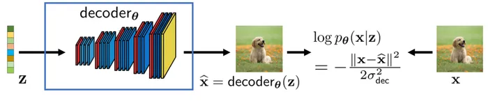
which measures the generative accuracy of the data point $x$ passing through the encoder $q(z|x)$ to yield high probability samples which are close to the original signal (data) $p^{\ast}(x)$.

Gaussian VAEs

Lets consider a simpel scenario of an VAE where the encoder and the decoder are given by Gaussian distributions

where the mean and covariances are now paramterized by a neural network, for example the mean as a vector and diagonal of the covariances. Taking the prior latent distribution $q(z) = \mathcal{N}(0,I)$ the evaluation of the (ELBO) is approximately achieved by\

• Sampling over the encoder distribution which is Gaussian and therefore tractable
• Evaluating the brackets within the expectation which are given in closed form solution

and

Thus we get

where we put all the contants undependent of $\theta,\phi$ into the constant $D$. Taking a minibatch $\mathcal{B}\subset \mathcal{D}$ of the training the parameters are then optimized by batch gradient descent

Forward Pass

Given a dataset of independently and identically distributed $i.i.d.$ data points $\qquad \qquad \qquad \qquad \qquad \qquad \mathcal{D}=\{{\mathbf{x}}^{(1)},{\mathbf{x}}^{(2)},...,{\mathbf{x}}^{(N)}\}\equiv\{{\mathbf{x}}^{(i)}\}_{i=1}^{N}$

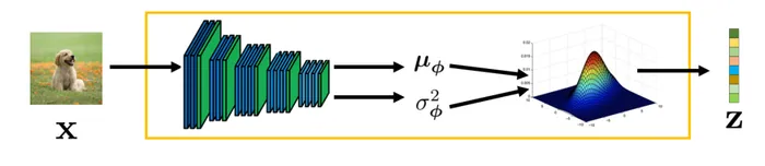
the optimization of the encoder decoder boilds down to the following steps. First Picking a random sample $x \in \mathcal{D}$ we need to pass the data through the encoder by sampling a latent variable $z im \mathcal{N}(\mu(\phi(x)),\Sigma(\phi(x)))$. This is
accomplished by taking a neural network and to pass the input data $x$ and output given by the mean and and covariance matrix $\mu(\phi(x)),\Sigma(\phi(x)) = NN_{\phi}(x)$. Subsequently, the sampling a latent variable $z$ is performed by applying tranformation mapping to gaussian white noise $\epsilon \sim \mathcal{N}(0,I)$ via

where the square root of the covariance matrix is obtain by applying Cholesky decomposition.

Following similar steps the sampled $z \in \mathbb{R}^{d_z}$ is passed as the input to the second neural network which parametrized the mean and covariance of the decoder distribution $\hat{x} \sim \mathcal{N}(\mu(\theta(z)),\Sigma(\theta(z)))$ with $\mu(\theta(z)),\Sigma(\theta(z)) = NN_{\theta}(z)$

Problem with naive Gradient Descent

Having performed the forward pass we need to evolve the variational paramters $\phi,\theta$ towards a local mimimum of the ELBO objective via gradient descent where the gradient with respect to $\phi$ and $\theta$ are respectivaly given by

which can be apprxomited by a one sample Monte Carlo estimator

As can be observed from the above formula, despite a simple Monte Carlo approximation there are no difficulties in accessing the gradient for the backward propagation of variational paramters $\theta$. However, this is not the case for the gradient with respect to the encoder

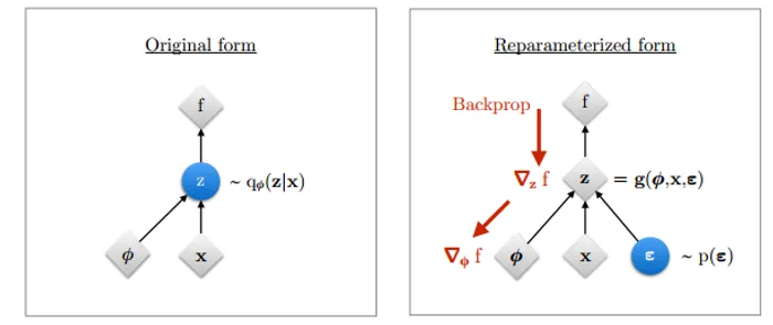
which is due to the neccecity to differentiate the expectation over $q_{\phi}(z|x)$ which is paramterized by $\phi$!. To tackle this problems we need to introduce the reparametrization trick.

Reparametrization Trick and Changes of Variables Formula

Concerning the problem of evaluating expression (todo) Rezende et al tackled the problem via the change of variables formula for continuous distributions

where $f_X$ and $f_Y$ denote probability densitity distributions respectivaly. To see why the above formula holds let us do some simple calculations given an invertible map $\Psi:Y \to X$ with $\det(\Psi)>0$. Because $\Psi$ maps random variables $y \in Y$ one to one to some $\Psi(y) \in X$ we first reexrpress the density $f_X$ to $f_Y$ using abbreviation $y(x) = \Psi^{-1}(x)$

where the fourth inequality holds due to positive determinant of the map $\Psi(y)$. Finally, applying the classical change of variables formula for intergrating multivariate functions with respect to substitution $y = \Psi^{-1}(x)$

Consider the following simple 1D exmaple with Gaussian distributed random variable $z \sim \mathcal{N}(z|0,1)$. Then the transformed term $x = \exp(z)$ is again a randmom variable with nonnegative derivative and using change of variable formula we know the density $f_X$ of $x$

$f_X(x)dx = \mathcal{N}(\log(x)|0,1)\cdot \frac{1}{x}dx$

as can be observed by the following figure

Using the change of variables we can reparametrize the expectation of $z$ in terms of standart Gaussian random variable $\epsilon = \mathcal{N}(0,I)$ by looking for a mapping $z = g(\epsilon,\phi,x)$ which yields with $f_x(z,\theta,\phi) = \log p_{\theta}(\mathbf{x},\mathbf{z})-\log q_{\phi}(\mathbf{z}|\mathbf{x})$

which equals $\mathbb{E}_{p(\epsilon)}\left[f({\bf z})\right]$. The important observation of the above reparametrization trick comes from the changed expectation from $z \sim q_{\phi}(z|x)$ that depends on $\phi$ to a simple standart Gaussian distribution $\mathcal{N}(\epsilon|0,I)$. Moreover this yields an efficient evaluation of the gradient with respect to the problematic variational paramter $\phi$

In other word reparamterization trick makes it possible backpropage through the encoder part of the network as can be observed from the following figure

For a one sample Monte Carlo estimator with $\epsilon \sim \mathcal{N}(0,I)$ and $z = g(\phi,x,\epsilon)$ evaluation of the ELBO amount to compute

$\hat{\mathcal{L}}_{\theta,\phi,\epsilon}({\bf x}) = \log p_{\theta}({\bf x},{\bf z})-\log q_{\phi}({\bf z}|{\bf x})$

which yields an unbiased estimator as can be observed from

$\mathbb{E}_{p(\epsilon)}\left[\nabla_{\theta,\phi}\hat{\mathcal{L}}_{\theta,\phi,\epsilon}({\bf x})\right]=\mathbb{E}_{p(\epsilon)}\left[\nabla_{\theta,\phi}(\log p\theta(\mathbf{x},\mathbf{z})-\log q_{\phi}(\mathbf{z}|\mathbf{x}))\right] =\nabla_{\theta,\phi}(\mathbb{E}_{p(\epsilon)}\left[\log p_{\theta}(\mathbf{x},\mathbf{z})-\log q_{\phi}(\mathbf{z}|\mathbf{x})\right]) = \nabla_{\theta,\phi}\mathcal{L}_{\theta,\phi}(x)$

i.e. the expected gradient with respect to white noise distribution $p(\epsilon)$ results in the exact expression of the truth gradient of the ELBO objective.

Lets next consider the building blog of evaluating the remaining parts of the one sample ELBO approximation.

• Calculation of encoder log probability $\log_{\phi}(z|x)$ given a data point $x \in \mathcal{D}$ mainly connects to the choice of a proper invertible mapping $z = g(\epsilon)$ and tractable density $p(\epsilon)$. Using the change of variables formula the computation boils down to

$\log q_{\phi}(z|x) = \log p(\epsilon)-\log|\det(\frac{\partial g(\epsilon)}{\partial \epsilon})|$

which in particular shows that tractable mappings are those which Jacobian is upper or lower triangular matrix where an important class of such mappings is given by assumming the mean-field like strucutre of the encoder

$q_{\phi}({\bf z}|{\bf x})=\prod_{i}q_{\phi}(z_{i}|{\bf x})=\prod_{i}N(z_{i};\mu_{i},\sigma_{i}^{2})$

Then the mapping $g(\epsilon)$ can be contructed from the transformation of gaussian distribution under linear transofmation, i.e. via

$\epsilon \sim \mathcal{N}(0,{\bf I}) \qquad \epsilon=\mathrm{NN_{Encoder}}\phi({\bf x}) \qquad z = g(\epsilon,\phi) = \mu+\sigma \odot\epsilon$

with Jacobian given by a simple diagonal matrix with covariance at the diagonal.

More generally, we can generalize the above case to $q_{\phi}(z|x) = \mathcal{N}(z|\mu(x),\Sigma(x))$ using Cholesky factorization $\Sigma(x) = LL^T$ with invertible mapping $g(\epsilon) = \mu+ L\epsilon$ with closed form of the encoder

$\log q_{\phi}(\mathbf{z}|\mathbf{x})=\log p(\epsilon)-\sum_{i}\log|L_{i i}|$

Hereby, the parametrization of $L$ in terms of neural network can be achieved in two steps

• First $(\mu,\log\sigma,\mathbf{L}^{\prime}) = \mathrm{NN_{Encoder}}_{\phi}(\mathbf{x})$
• Second, applying a masking matrix $L_{mask}$ with zeros above the diagonal via ${\bf L} = {\bf L}_{m a s k} \odot {\bf L}^{\prime}+\mathrm{diag}(\sigma)$.

Chalenges

• The model can be trapped within undesirable stable equilibrium which happens when in the first optimization steps $p(x|z)$ is low and $q_{\phi}(z|x) \approx p(z)$
• Blurriness Artifacts for nonzero KL-divergence between $q_{\phi}(x,z)$ and $p_{\theta}(x,z)$ which causes the variance of the decoder $p_{\theta}(x,z)$ to be higher then variance of the encoder $q_{\phi}(z,x)$ and the data $q_{\phi}(x)$